分析01

実データ 01_Data/ に対して適用する

dow_jones_index

https://archive.ics.uci.edu/dataset/312/dow+jones+index

This dataset contains weekly data for the Dow Jones Industrial Index. It has been used in computational investing research.

項目名	説明
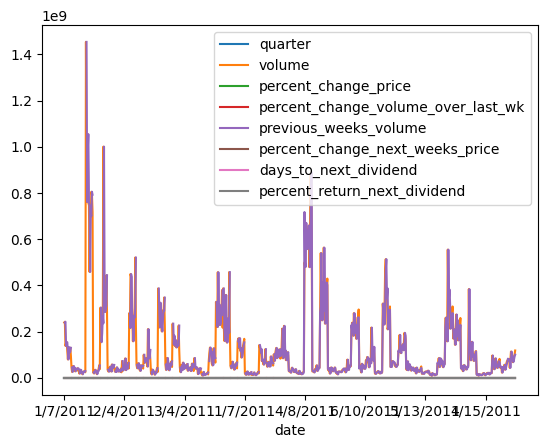
quarter	年間の四半期（1 = 1〜3月、2 = 4〜6月）
stock	株式のシンボル（ティッカーコード）
date	週の最終営業日（通常は金曜日）
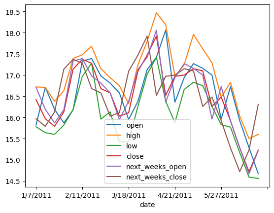
open	週の始めの株価（始値）
high	週の最高株価
low	週の最安株価
close	週の終わりの株価（終値）
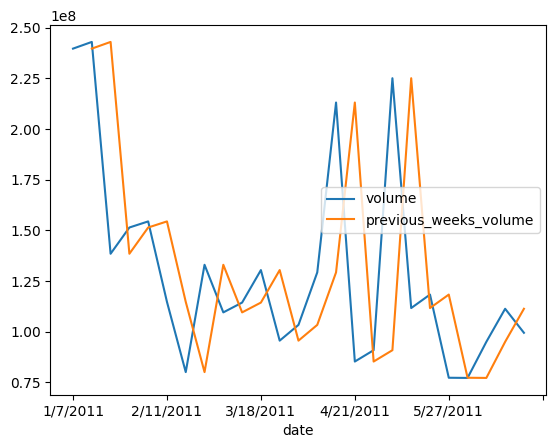
volume	その週に取引された株式の出来高（取引株数）
percent_change_price	週を通しての株価変動率（％）
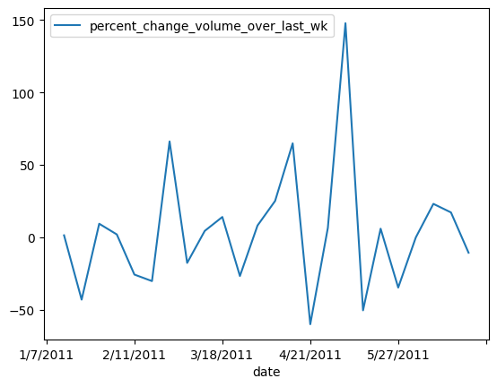
percent_change_volume_over_last_week	前週と比較した出来高の変化率（％）
previous_weeks_volume	前週の出来高（取引株数）
next_weeks_open	翌週の始値
next_weeks_close	翌週の終値
percent_change_next_weeks_price	翌週の株価変動率（％）
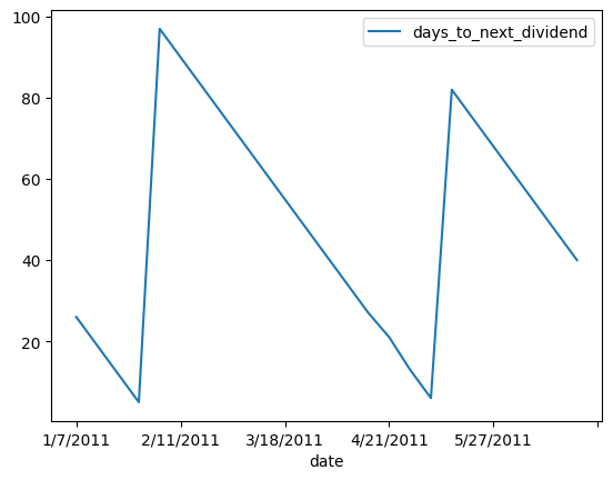
days_to_next_dividend	次回配当までの日数
percent_return_next_dividend	次回配当による利回り（％）

df = pd.read_csv("01_Data/dow_jones_index/dow_jones_index.data")
df

	quarter	stock	date	open	high	low	close	volume	percent_change_price	percent_change_volume_over_last_wk	previous_weeks_volume	next_weeks_open	next_weeks_close	percent_change_next_weeks_price	days_to_next_dividend	percent_return_next_dividend
0	1	AA	1/7/2011	$15.82	$16.72	$15.78	$16.42	239655616	3.79267	NaN	NaN	$16.71	$15.97	-4.428490	26	0.182704
1	1	AA	1/14/2011	$16.71	$16.71	$15.64	$15.97	242963398	-4.42849	1.380223	239655616.0	$16.19	$15.79	-2.470660	19	0.187852
2	1	AA	1/21/2011	$16.19	$16.38	$15.60	$15.79	138428495	-2.47066	-43.024959	242963398.0	$15.87	$16.13	1.638310	12	0.189994
3	1	AA	1/28/2011	$15.87	$16.63	$15.82	$16.13	151379173	1.63831	9.355500	138428495.0	$16.18	$17.14	5.933250	5	0.185989
4	1	AA	2/4/2011	$16.18	$17.39	$16.18	$17.14	154387761	5.93325	1.987452	151379173.0	$17.33	$17.37	0.230814	97	0.175029
...	...	...	...	...	...	...	...	...	...	...	...	...	...	...	...	...
745	2	XOM	5/27/2011	$80.22	$82.63	$80.07	$82.63	68230855	3.00424	-21.355713	86758820.0	$83.28	$81.18	-2.521610	75	0.568801
746	2	XOM	6/3/2011	$83.28	$83.75	$80.18	$81.18	78616295	-2.52161	15.221032	68230855.0	$80.93	$79.78	-1.420980	68	0.578960
747	2	XOM	6/10/2011	$80.93	$81.87	$79.72	$79.78	92380844	-1.42098	17.508519	78616295.0	$80.00	$79.02	-1.225000	61	0.589120
748	2	XOM	6/17/2011	$80.00	$80.82	$78.33	$79.02	100521400	-1.22500	8.811952	92380844.0	$78.65	$76.78	-2.377620	54	0.594786
749	2	XOM	6/24/2011	$78.65	$81.12	$76.78	$76.78	118679791	-2.37762	18.064204	100521400.0	$76.88	$82.01	6.672740	47	0.612139

750 rows × 16 columns

df1 = df.set_index("date")
df1

	quarter	stock	open	high	low	close	volume	percent_change_price	percent_change_volume_over_last_wk	previous_weeks_volume	next_weeks_open	next_weeks_close	percent_change_next_weeks_price	days_to_next_dividend	percent_return_next_dividend
date
1/7/2011	1	AA	$15.82	$16.72	$15.78	$16.42	239655616	3.79267	NaN	NaN	$16.71	$15.97	-4.428490	26	0.182704
1/14/2011	1	AA	$16.71	$16.71	$15.64	$15.97	242963398	-4.42849	1.380223	239655616.0	$16.19	$15.79	-2.470660	19	0.187852
1/21/2011	1	AA	$16.19	$16.38	$15.60	$15.79	138428495	-2.47066	-43.024959	242963398.0	$15.87	$16.13	1.638310	12	0.189994
1/28/2011	1	AA	$15.87	$16.63	$15.82	$16.13	151379173	1.63831	9.355500	138428495.0	$16.18	$17.14	5.933250	5	0.185989
2/4/2011	1	AA	$16.18	$17.39	$16.18	$17.14	154387761	5.93325	1.987452	151379173.0	$17.33	$17.37	0.230814	97	0.175029
...	...	...	...	...	...	...	...	...	...	...	...	...	...	...	...
5/27/2011	2	XOM	$80.22	$82.63	$80.07	$82.63	68230855	3.00424	-21.355713	86758820.0	$83.28	$81.18	-2.521610	75	0.568801
6/3/2011	2	XOM	$83.28	$83.75	$80.18	$81.18	78616295	-2.52161	15.221032	68230855.0	$80.93	$79.78	-1.420980	68	0.578960
6/10/2011	2	XOM	$80.93	$81.87	$79.72	$79.78	92380844	-1.42098	17.508519	78616295.0	$80.00	$79.02	-1.225000	61	0.589120
6/17/2011	2	XOM	$80.00	$80.82	$78.33	$79.02	100521400	-1.22500	8.811952	92380844.0	$78.65	$76.78	-2.377620	54	0.594786
6/24/2011	2	XOM	$78.65	$81.12	$76.78	$76.78	118679791	-2.37762	18.064204	100521400.0	$76.88	$82.01	6.672740	47	0.612139

750 rows × 15 columns

df1.plot()

• x quarter

dol_cols = [
  "open", 
  "high", 
  "low", 
  "close", 
  "next_weeks_open", 
  "next_weeks_close"
  ]

df1[dol_cols] = (
    df1[dol_cols]
    .replace('[\$,]', '', regex=True)  # $, , を削除
    .astype(float)                     # float型に変換
)

df1

	quarter	stock	open	high	low	close	volume	percent_change_price	percent_change_volume_over_last_wk	previous_weeks_volume	next_weeks_open	next_weeks_close	percent_change_next_weeks_price	days_to_next_dividend	percent_return_next_dividend
date
1/7/2011	1	AA	15.82	16.72	15.78	16.42	239655616	3.79267	NaN	NaN	16.71	15.97	-4.428490	26	0.182704
1/14/2011	1	AA	16.71	16.71	15.64	15.97	242963398	-4.42849	1.380223	239655616.0	16.19	15.79	-2.470660	19	0.187852
1/21/2011	1	AA	16.19	16.38	15.60	15.79	138428495	-2.47066	-43.024959	242963398.0	15.87	16.13	1.638310	12	0.189994
1/28/2011	1	AA	15.87	16.63	15.82	16.13	151379173	1.63831	9.355500	138428495.0	16.18	17.14	5.933250	5	0.185989
2/4/2011	1	AA	16.18	17.39	16.18	17.14	154387761	5.93325	1.987452	151379173.0	17.33	17.37	0.230814	97	0.175029
...	...	...	...	...	...	...	...	...	...	...	...	...	...	...	...
5/27/2011	2	XOM	80.22	82.63	80.07	82.63	68230855	3.00424	-21.355713	86758820.0	83.28	81.18	-2.521610	75	0.568801
6/3/2011	2	XOM	83.28	83.75	80.18	81.18	78616295	-2.52161	15.221032	68230855.0	80.93	79.78	-1.420980	68	0.578960
6/10/2011	2	XOM	80.93	81.87	79.72	79.78	92380844	-1.42098	17.508519	78616295.0	80.00	79.02	-1.225000	61	0.589120
6/17/2011	2	XOM	80.00	80.82	78.33	79.02	100521400	-1.22500	8.811952	92380844.0	78.65	76.78	-2.377620	54	0.594786
6/24/2011	2	XOM	78.65	81.12	76.78	76.78	118679791	-2.37762	18.064204	100521400.0	76.88	82.01	6.672740	47	0.612139

750 rows × 15 columns

df1.groupby("stock").count()

	quarter	open	high	low	close	volume	percent_change_price	percent_change_volume_over_last_wk	previous_weeks_volume	next_weeks_open	next_weeks_close	percent_change_next_weeks_price	days_to_next_dividend	percent_return_next_dividend
stock
AA	25	25	25	25	25	25	25	24	24	25	25	25	25	25
AXP	25	25	25	25	25	25	25	24	24	25	25	25	25	25
BA	25	25	25	25	25	25	25	24	24	25	25	25	25	25
BAC	25	25	25	25	25	25	25	24	24	25	25	25	25	25
CAT	25	25	25	25	25	25	25	24	24	25	25	25	25	25
CSCO	25	25	25	25	25	25	25	24	24	25	25	25	25	25
CVX	25	25	25	25	25	25	25	24	24	25	25	25	25	25
DD	25	25	25	25	25	25	25	24	24	25	25	25	25	25
DIS	25	25	25	25	25	25	25	24	24	25	25	25	25	25
GE	25	25	25	25	25	25	25	24	24	25	25	25	25	25
HD	25	25	25	25	25	25	25	24	24	25	25	25	25	25
HPQ	25	25	25	25	25	25	25	24	24	25	25	25	25	25
IBM	25	25	25	25	25	25	25	24	24	25	25	25	25	25
INTC	25	25	25	25	25	25	25	24	24	25	25	25	25	25
JNJ	25	25	25	25	25	25	25	24	24	25	25	25	25	25
JPM	25	25	25	25	25	25	25	24	24	25	25	25	25	25
KO	25	25	25	25	25	25	25	24	24	25	25	25	25	25
KRFT	25	25	25	25	25	25	25	24	24	25	25	25	25	25
MCD	25	25	25	25	25	25	25	24	24	25	25	25	25	25
MMM	25	25	25	25	25	25	25	24	24	25	25	25	25	25
MRK	25	25	25	25	25	25	25	24	24	25	25	25	25	25
MSFT	25	25	25	25	25	25	25	24	24	25	25	25	25	25
PFE	25	25	25	25	25	25	25	24	24	25	25	25	25	25
PG	25	25	25	25	25	25	25	24	24	25	25	25	25	25
T	25	25	25	25	25	25	25	24	24	25	25	25	25	25
TRV	25	25	25	25	25	25	25	24	24	25	25	25	25	25
UTX	25	25	25	25	25	25	25	24	24	25	25	25	25	25
VZ	25	25	25	25	25	25	25	24	24	25	25	25	25	25
WMT	25	25	25	25	25	25	25	24	24	25	25	25	25	25
XOM	25	25	25	25	25	25	25	24	24	25	25	25	25	25

numcols = ["open", "high", "low", "close", "volume", "percent_change_price", "percent_change_volume_over_last_wk", "previous_weeks_volume", "next_weeks_open", "next_weeks_close", "percent_change_next_weeks_price", "days_to_next_dividend", "percent_return_next_dividend"]
dfAA = df1[df1["stock"] == "AA"][numcols]
dfAA

	open	high	low	close	volume	percent_change_price	percent_change_volume_over_last_wk	previous_weeks_volume	next_weeks_open	next_weeks_close	percent_change_next_weeks_price	days_to_next_dividend	percent_return_next_dividend
date
1/7/2011	15.82	16.72	15.78	16.42	239655616	3.792670	NaN	NaN	16.71	15.97	-4.428490	26	0.182704
1/14/2011	16.71	16.71	15.64	15.97	242963398	-4.428490	1.380223	239655616.0	16.19	15.79	-2.470660	19	0.187852
1/21/2011	16.19	16.38	15.60	15.79	138428495	-2.470660	-43.024959	242963398.0	15.87	16.13	1.638310	12	0.189994
1/28/2011	15.87	16.63	15.82	16.13	151379173	1.638310	9.355500	138428495.0	16.18	17.14	5.933250	5	0.185989
2/4/2011	16.18	17.39	16.18	17.14	154387761	5.933250	1.987452	151379173.0	17.33	17.37	0.230814	97	0.175029
2/11/2011	17.33	17.48	16.97	17.37	114691279	0.230814	-25.712195	154387761.0	17.39	17.28	-0.632547	90	0.172712
2/18/2011	17.39	17.68	17.28	17.28	80023895	-0.632547	-30.226696	114691279.0	16.98	16.68	-1.766780	83	0.173611
2/25/2011	16.98	17.15	15.96	16.68	132981863	-1.766780	66.177694	80023895.0	16.81	16.58	-1.368230	76	0.179856
3/4/2011	16.81	16.94	16.13	16.58	109493077	-1.368230	-17.663150	132981863.0	16.58	16.03	-3.317250	69	0.180941
3/11/2011	16.58	16.75	15.42	16.03	114332562	-3.317250	4.419900	109493077.0	15.95	16.11	1.003130	62	0.187149
3/18/2011	15.95	16.33	15.43	16.11	130374108	1.003130	14.030601	114332562.0	16.38	17.09	4.334550	55	0.186220
3/25/2011	16.38	17.24	16.26	17.09	95550392	4.334550	-26.710607	130374108.0	17.13	17.47	1.984820	48	0.175541
4/1/2011	17.13	17.80	17.02	17.47	103320396	1.984820	8.131839	95550392.0	17.42	17.92	2.870260	41	0.171723
4/8/2011	17.42	18.47	17.42	17.92	129237024	2.870260	25.083748	103320396.0	18.06	16.52	-8.527130	34	0.167411
4/15/2011	18.06	18.19	16.38	16.52	213061090	-8.527130	64.860721	129237024.0	16.36	16.97	3.728610	27	0.181598
4/21/2011	16.36	16.97	15.88	16.97	85235391	3.728610	-59.994858	213061090.0	16.94	17.00	0.354191	21	0.176783
4/29/2011	16.94	17.24	16.66	17.00	90831895	0.354191	6.565939	85235391.0	17.27	17.15	-0.694847	13	0.176471
5/6/2011	17.27	17.96	16.83	17.15	225053559	-0.694847	147.769309	90831895.0	17.16	17.10	-0.349650	6	0.174927
5/13/2011	17.16	17.62	16.75	17.10	111630753	-0.349650	-50.398139	225053559.0	17.00	16.26	-4.352940	82	0.175439
5/20/2011	17.00	17.29	16.26	16.26	118281015	-4.352940	5.957374	111630753.0	15.96	16.48	3.258150	75	0.184502
5/27/2011	15.96	16.48	15.83	16.48	77236662	3.258150	-34.700711	118281015.0	16.73	15.92	-4.841600	68	0.182039
6/3/2011	16.73	16.83	15.77	15.92	77152591	-4.841600	-0.108849	77236662.0	15.92	15.28	-4.020100	61	0.188442
6/10/2011	15.92	16.03	15.17	15.28	94970970	-4.020100	23.094985	77152591.0	15.29	14.72	-3.727930	54	0.196335
6/17/2011	15.29	15.50	14.59	14.72	111273573	-3.727930	17.165880	94970970.0	14.67	15.23	3.817310	47	0.203804
6/24/2011	14.67	15.60	14.56	15.23	99423717	3.817310	-10.649299	111273573.0	15.22	16.31	7.161630	40	0.196980

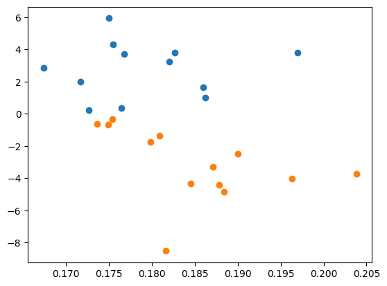
cols1 = ["open", "high", "low", "close", "next_weeks_open", "next_weeks_close"]
cols2 = ["volume", "previous_weeks_volume"]
cols3 = ["percent_change_price", "percent_change_next_weeks_price"]
cols4 = ["percent_change_volume_over_last_wk"]
cols5 = ["days_to_next_dividend"]
cols6 = ["percent_return_next_dividend"]

dfAA[cols1].plot()

dfAA[cols2].plot()

dfAA[cols3].plot()

dfAA[cols4].plot()

dfAA[cols5].plot()

dfAA[cols6].plot()

True: 上がる、False: 下がる

dfAA["open_updown"] = dfAA["open"] < dfAA["next_weeks_open"]
dfAA["close_updown"] = dfAA["close"] < dfAA["next_weeks_close"]

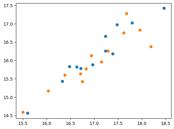
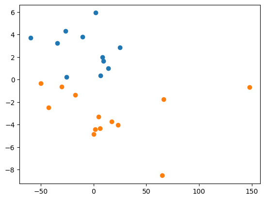
up = dfAA[dfAA["open_updown"]]
down = dfAA[~dfAA["open_updown"]]
plt.scatter(x = up["high"], y = up["low"])
plt.scatter(x = down["high"], y = down["low"])

plt.scatter(x = up[cols3[0]], y = up[cols2[0]])
plt.scatter(x = down[cols3[0]], y = down[cols2[0]])

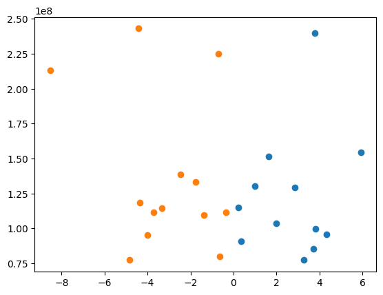
plt.scatter(x = up[cols6[0]], y = up[cols2[0]])
plt.scatter(x = down[cols6[0]], y = down[cols2[0]])

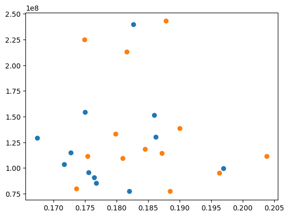
plt.scatter(x = up[cols6[0]], y = up[cols3[0]])
plt.scatter(x = down[cols6[0]], y = down[cols3[0]])

plt.scatter(x = up[cols4[0]], y = up[cols3[0]])
plt.scatter(x = down[cols4[0]], y = down[cols3[0]])

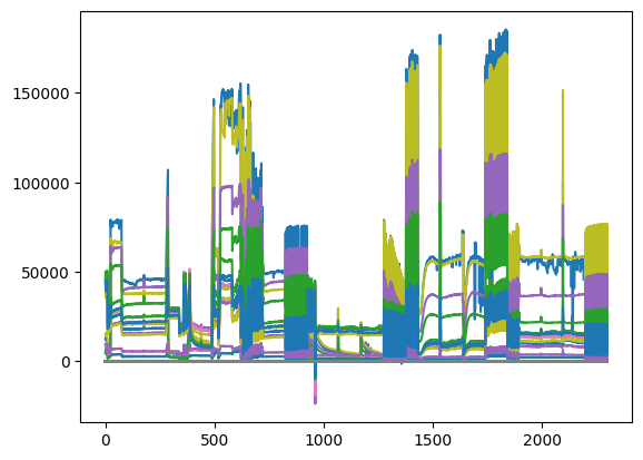
def load_custom_file(filepath):
    data = []

    with open(filepath, 'r') as f:
        for line in f:
            parts = line.strip().split()
            label = parts[0]  # 最初の数字（ラベル部分）

            # 残りの "番号:値" ペアを辞書に変換
            features = {}
            for item in parts[1:]:
                idx, val = item.split(':')
                features[int(idx)] = float(val)

            # ラベルを追加
            features['label'] = label
            data.append(features)

    # DataFrameに変換（欠けているカラムはNaNで埋める）
    df = pd.DataFrame(data)

    # カラム順を label → feature1, feature2, ...
    cols = ['label'] + sorted([c for c in df.columns if c != 'label'])
    df = df[cols]

    return df

DF = load_custom_file("01_Data/Gas Sensor Array Drift Dataset/batch6.dat")
DF.plot(legend=None)

df = pd.read_csv(
    "01_Data/secom/secom_labels.data",
    sep=r'\s+',
    quotechar='"',
    names=['label', 'timestamp']
)
df['timestamp'] = pd.to_datetime(df['timestamp'], format='%d/%m/%Y %H:%M:%S')
df

	label	timestamp
0	-1	2008-07-19 11:55:00
1	-1	2008-07-19 12:32:00
2	1	2008-07-19 13:17:00
3	-1	2008-07-19 14:43:00
4	-1	2008-07-19 15:22:00
...	...	...
1562	-1	2008-10-16 15:13:00
1563	-1	2008-10-16 20:49:00
1564	-1	2008-10-17 05:26:00
1565	-1	2008-10-17 06:01:00
1566	-1	2008-10-17 06:07:00

1567 rows × 2 columns

df1 = pd.read_csv("01_Data/secom/secom.data", sep=r'\s+', header=None)
df1

	0	1	2	3	4	5	6	7	8	9	...	580	581	582	583	584	585	586	587	588	589
0	3030.93	2564.00	2187.7333	1411.1265	1.3602	100.0	97.6133	0.1242	1.5005	0.0162	...	NaN	NaN	0.5005	0.0118	0.0035	2.3630	NaN	NaN	NaN	NaN
1	3095.78	2465.14	2230.4222	1463.6606	0.8294	100.0	102.3433	0.1247	1.4966	-0.0005	...	0.0060	208.2045	0.5019	0.0223	0.0055	4.4447	0.0096	0.0201	0.0060	208.2045
2	2932.61	2559.94	2186.4111	1698.0172	1.5102	100.0	95.4878	0.1241	1.4436	0.0041	...	0.0148	82.8602	0.4958	0.0157	0.0039	3.1745	0.0584	0.0484	0.0148	82.8602
3	2988.72	2479.90	2199.0333	909.7926	1.3204	100.0	104.2367	0.1217	1.4882	-0.0124	...	0.0044	73.8432	0.4990	0.0103	0.0025	2.0544	0.0202	0.0149	0.0044	73.8432
4	3032.24	2502.87	2233.3667	1326.5200	1.5334	100.0	100.3967	0.1235	1.5031	-0.0031	...	NaN	NaN	0.4800	0.4766	0.1045	99.3032	0.0202	0.0149	0.0044	73.8432
...	...	...	...	...	...	...	...	...	...	...	...	...	...	...	...	...	...	...	...	...	...
1562	2899.41	2464.36	2179.7333	3085.3781	1.4843	100.0	82.2467	0.1248	1.3424	-0.0045	...	0.0047	203.1720	0.4988	0.0143	0.0039	2.8669	0.0068	0.0138	0.0047	203.1720
1563	3052.31	2522.55	2198.5667	1124.6595	0.8763	100.0	98.4689	0.1205	1.4333	-0.0061	...	NaN	NaN	0.4975	0.0131	0.0036	2.6238	0.0068	0.0138	0.0047	203.1720
1564	2978.81	2379.78	2206.3000	1110.4967	0.8236	100.0	99.4122	0.1208	NaN	NaN	...	0.0025	43.5231	0.4987	0.0153	0.0041	3.0590	0.0197	0.0086	0.0025	43.5231
1565	2894.92	2532.01	2177.0333	1183.7287	1.5726	100.0	98.7978	0.1213	1.4622	-0.0072	...	0.0075	93.4941	0.5004	0.0178	0.0038	3.5662	0.0262	0.0245	0.0075	93.4941
1566	2944.92	2450.76	2195.4444	2914.1792	1.5978	100.0	85.1011	0.1235	NaN	NaN	...	0.0045	137.7844	0.4987	0.0181	0.0040	3.6275	0.0117	0.0162	0.0045	137.7844

1567 rows × 590 columns